Chapter 2 The Backprop Algorithm

Copyright by Donald R. Tveter

http://www.dontveter.com, http://www.dontveter.com/email.html

Commercial Use Prohibited

2.1  Evaluating a Network

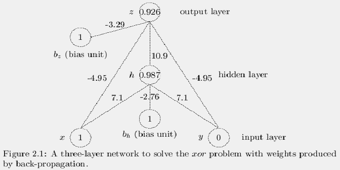
Figure 2.1 shows a simple back-propagation network that computes the exclusive-or (xor) of two inputs, x and y. The xor function, z = xor(x,y) is defined as follows:

x y z 1 0 1 0 0 0 0 1 1 1 1 0

In this figure the circles represent neurons or units or nodes that are extremely simple analog computing devices. The numbers within the circles represent the activation values of the units. The main nodes are arranged in layers. In this case there are three layers, the input layer that contains the values for x and y, a hidden layer that contains one node, h and an output unit that gives the value of the output value, z. The hidden layer is so-named because the network can be regarded as a black box with inputs and outputs that can be seen but the hidden units cannot be seen. There are two other units present called bias units whose values are always 1.0. For now we are not going to claim that they are part of any one layer. Most of the time when a network is drawn the bias units are not even shown. When other writers want to emphasize the presence of a bias unit there is often only one unit shown in the diagram of the network and that one unit is used for the entire network. This is probably the only example where we will show the bias units at all. The lines connecting the circles represent weights and the number beside a weight is the value of the weight. Much of the time back-propagation networks only have connections within adjacent layers however this one has two extra connections that go directly from the input units to the output unit. In some problems, like xor these extra input-output connections make training the network much faster. Networks are usually just described by the number of units in each layer so the network in 2.1 can be described as a 2-1-1 network with extra input-output connections. In this report this will be shortened to 2-1-1-x.

To compute the value of the output unit, z, we place values for x and y on the input layer units. Let these values be 1.0 and 0.0 as in figure 2.1. First we compute the value of the hidden layer unit, h. The first step of this computation is to look at each lower level unit and the bias unit that is connected to the hidden unit. For each of these connections, find the value of the unit and multiply by the weight and sum all the results. The calculations give:

1.0 * 7.1 = 7.10 1.0 * -2.76 = -2.76 0.0 * 7.1 = 0.00 sum = 4.34

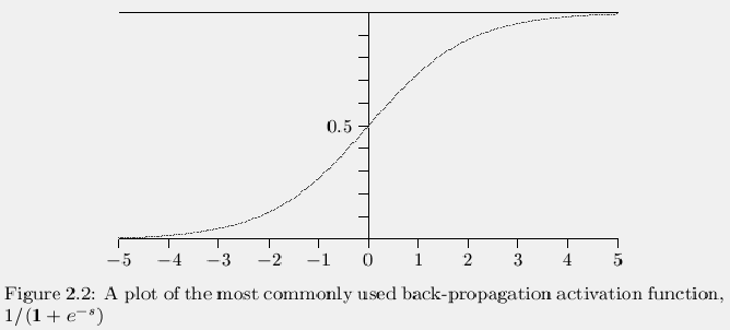
In some neural networks we might just leave the activation value of the unit to be 4.34. In this case we would say that we are using the linear activation function, however backprop is at its best when this value is passed to certain types of non-linear functions. The most commonly used non-linear function is:

v = 1 1+e-s

where s is the sum of the inputs to the neuron and v is the value of the neuron. Thus, with s = 4.34, v = 0.987. This particular function will be called the standard sigmoid in this manual. Quite often it is called the logistic function. The general function used to compute the value of a neuron can be called the activation function , squashing function or transfer function . The calculations for the output unit, z are:

1.000 * -4.95 = -4.95 0.000 * -4.95 = 0.00 0.987 * 10.9 = 10.76 1.000 * -3.29 = -3.29 sum = 2.52 v = 0.926

Of course, 0.926 is not quite 1 but for this example it is close enough. When using this particular activation function for a problem where the output is supposed to be a 0 or 1 getting the output to within 0.1 of the target value is a very common standard but other people may want to get to closer than this while others don't want to get even this close. With this particular activation function it is actually somewhat hard to get very close to 1 or 0 because the function only approaches 1 and 0 as the input to the function approaches ¥ and -¥. Figure 2.2 shows a graph of the function with the y direction stretched with respect to the x direction. There are other activation functions you can use that make it easier to get closer to the exact targets. The other values the network computes for the xor function are:

x y z 1 0 0.926 0 0 0.067 0 1 0.926 1 1 0.092

The formulas for computing the activation value for a neuron, j can be written more concisely as follows. Let the activation value for neuron j be o_j. Let the activation function be the general function, f. Let the weight between neuron j and neuron i be w_ij. Let the net input to neuron j be net_j, then

netj = å i = 1,n  wijoi

(2.1)

where n is the number of units feeding into unit j and

oj = f(netj)

(2.2)

2.2  Training a Network

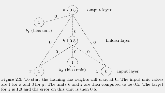
Figure 2.3 shows a 2-1-1-x xor network before it has been trained to compute the xor function. In this example the network weights will all start out at 0 (a bad idea in general but it works here) and the training process will try to adjust the weights so that the answers come out right. It will work as follows. First put one of the patterns to be learned on the input units. Second, find the values for the hidden unit and output unit. Third, find out how large the error is on the output unit. Fourth, use one of the back-propagation formulas to adjust the weights leading into the output unit. The idea is to try to make the answer come out just a little bit closer to the right answer. Fifth, use another formula to find out errors for the hidden layer unit. Sixth, adjust the weights leading into the hidden layer unit via another formula. Repeat steps one thru six for the second, third and fourth xor patterns. Even after all these changes to the weights the answers will only be a little closer to the right answers and the whole process has to be repeated many times. Each time all the patterns in the problem have been used once we will call that an iteration although often other people call this an epoch .

We will now look at the formulas for adjusting the weights that lead into the output units of a back-propagation network. The actual activation value of an output unit, k, will be o_k and the target for unit, k, will be t_k. First of all there is a term in the formula for d_k, the error signal :

dk = (tk - ok)f¢(netk).

(2.3)

where f¢ is the derivative of the activation function, f. If we use the usual activation function:

1 1 + e-netk

the derivative term is:

ok(1-ok).

(2.4)

 The formula to change the weight, w_jk between the output unit, k, and unit j is:

wjk ¬ wjk + hdk oj

(2.5)

where h is some relatively small positive constant called the learning rate . With the network in 2.3 with h = 0.1 we have:

dz = (1 - 0.5) * 0.5 * (1 - 0.5) = 0.125

wzx ¬ 0 + 0.1 * 0.125 * 1 = 0.0125

wzy ¬ 0 + 0.1 * 0.125 * 0 = 0

wzh ¬ 0 + 0.1 * 0.125 * 0.5 = 0.00625

wzbz ¬ 0 + 0.1 * 0.125 * 1 = 0.0125

The formula for computing the error d_j for a hidden unit, j, is:

dj = f¢(netj) å k  dk wkj.

The k subscript is for all the units in the output layer however in this example there is only one unit. In the example, then:

dh = oh(1-oh) dz wzh

dh = 0.5 * (1 - 0.5) * 0.125 * 0.0.00625 = 0.000195313.

The weight change formula for a weight, w_ij that goes between the hidden unit, j and the input unit, i is essentially the same as before:

wij ¬ wij + hdj oi.

The new weights will be:

whx ¬ 0 + 0.1 * 0.000195313 * 1 = 0.0000195313

why ¬ 0 + 0.1 * 0.000195313 * 0 = 0

whbh ¬ 0 + 0.1 * 0.000195313 * 1 = 0.0000195313

The activation value for the output layer will now be 0.507031. If we now do the same for the other three patterns the output will be:

x y zdesired zactual 1 0 1 0.499830 0 0 0 0.499893 0 1 1 0.499830 1 1 0 0.499768

Sad to say but to get the outputs to within 0.1 requires 20,862 iterations, a very long time especially for such a short problem.

Fortunately there are a large number of things that can be done to speed-up the training and the time to do the xor problem can be reduced to around 12-20 iterations or so. The very simplest thing to do is to increase the learning rate, h. The following table shows how many iterations are used for different values of h.

h iterations 0.1 20,862 0.5 2,455 1.0 1,060 2.0 480 3.0 (fails)

Another unfortunate problem with backprop is that when the learning rate is too large the training can fail as it did in the case when h = 3.0. Here, after 10,000 iterations the results were:

x y zdesired zactual 1 0 1 0.994 0 0 0 0.009 0 1 1 0.994 1 1 0 1.000

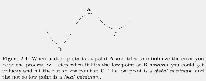
where the output for the last pattern is 1 not 0. The geometric interpretation of this problem is that when the network tries to make the error go down the network may get stuck in a valley that is not the lowest possible valley. For instance, suppose the error landscape is like the one shown in figure 2.4. There is one valley on the left that solves the problem but there is a shallower valley on the right that only gets some of the output values correct. This shallower valley is called a local minimum and the valley that gives the perfect results is called a global minimum , that is the best minimum that you can find. Once you go down into the shallow valley, if there is no path downhill that will get you to the deeper valley you are permanently stuck with a bad answer. There are ways to break out of a local minimum but in real world problems you never know when you've found the best (global) minimum, you only hope to get a very deep minimum.

The above method for changing the weights is actually a little less orthodox than most Mathematicians can accept. The problem is that when we used the first pattern we immediately changed the weight w_zh and used the changed weight to compute d_h. Many Mathematicians regard this as wrong but it works anyway. Instead they normally say that the weight changes can be computed but none of them should take effect until all the weight changes have been computed. The calculations then work as follows. First the error for the output unit is computed. The formula is:

dk = (tk - ok) ok (1 - ok)

and the calculation is:

dz = (1 - 0.5) * 0.5 * (1 - 0.5) = 0.125.

Next the weight changes for units leading into the output layer are done with the formula:

Dwjk = hdk oj

giving the calculations:

Dwzx = 0.1 * 0.125 * 1 = 0.0125

Dwzy = 0.1 * 0.125 * 0 = 0

Dwzh = 0.1 * 0.125 * 0.5 = 0.00625

Dwzbz = 0.1 * 0.125 * 1 = 0.0125

Now the error for the hidden layer unit is computed using the formala:

dj = oj(1-oj) å k  dk wkj

and this gives the calculation:

dh = 0.5 * (1 - 0.5) * 0.125 * 0 = 0

The weight change formula is again:

Dwij = hdj oi

This gives the calculations:

Dwhx = 0.1 * 0 * 1 = 0

Dwhy = 0.1 * 0 * 0 = 0

Dwhbh = 0.1 * 0 * 1 = 0

Now the weight changes are applied:

wzx ¬ wzx + Dwzx = 0 + 0.0125 = 0.0125

wzy ¬ wzy + Dwzy = 0 + 0 = 0

wzh ¬ wzh + Dwzh = 0 + 0.00625 = 0.00625

wzbz ¬ wzbz + Dwzbz = 0 + 0.0125 = 0.0125

whx ¬ whx + Dwhx = 0 + 0 = 0

why ¬ why + Dwhy = 0 + 0 = 0

whbh ¬ whbh + Dwhbh = 0 + 0 = 0

In this case it requires 25,496 iterations to get to within 0.1 of the targets. In fact the ``wrong" method is sometimes a little faster on some problems than the ``right" method although sometimes the ``right" method is better. Again, learning can be made faster by increasing h, but only to a point, as the data in the following table shows:

h iterations 0.1 25,496 0.5 3,172 1.0 1,381 2.0 617 3.0 391 4.0 (fails)

Both of the above methods for changing the weights are called online or continuous update methods because the changes are applied after each pattern is presented. To distinguish between the two in this report they will be the ``wrong" and the ``right" or ``correct" continuous update methods. There is a third alternative, the batch or periodic update method. In this method the weight changes for each weight are added up for every pattern and after all the patterns have made their contributions the weights are changed only once. Thus with the four patterns in the xor problem the weights are changed only once for each iteration rather than 4 times as in either of the continuous update methods. This means that less arithmetic needs to be done each iteration and each iteration is therefore slightly faster. On the other hand the continuous methods do more weight changes and take more time per iteration but they normally require fewer iterations. I can't give you an example just now of how long it takes to do the xor problem with periodic updates because when the initial weights are all 0 the weight changes all cancel out and no learning takes place. This doesn't happen in most problems but in all problems the network converges faster when the weights start out with small random values, a subject coming up soon.

A second variation on the periodic update method is to update more than once for each iteration after just a fixed number of patterns are processed. So if there were 1000 patterns to be learned an update might happen every 100 patterns.

In some implementations of backprop the learning rate h for periodic updates is automatically divided by the number of patterns. In this software it is NOT.

2.3  A Derivation of Backprop

No text on backprop would be complete without a derivation of the formulas so in this section they will be derived. Anyone with Math Anxiety can skip this section without missing a thing.

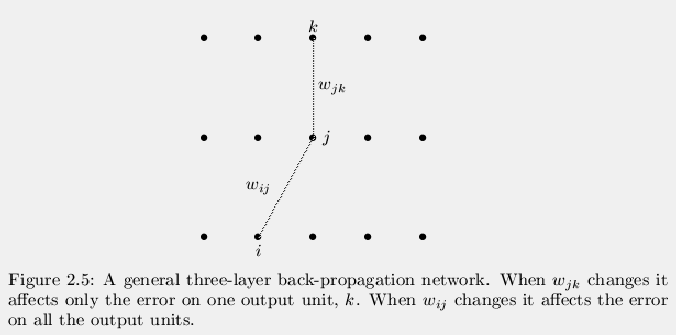
Figure 2.5 shows a general three layer network. In this network, the following relationships hold:

ok = 1 1 + e-netk

netk = å j  wjk oj

oj = 1 1 + e-netj

netj = å i  wijoi

Backprop is derived by assuming you want to minimize the error on the output units over all the patterns using the following formula for this error, E:

E = 1 2 å p  ( å k  (tpk - opk)2)

where p is the subscript for the pattern and k is the subscript for the output units. Then, t_pk is the target value of output unit k for pattern p and o_pk is the actual output value of output layer unit k for pattern p. This is by far the most commonly used error function however from time to time people have tried other error functions. Notice that E is the sum over all the patterns however we will assume that by minimizing the error for each pattern individually E will also be minimized. Therefore we will drop the subscript, p, from here on out and assume we are deriving the weight change formulas for just one pattern.

The first part of the problem is to find how E changes as the weight, w_jk, leading into an output unit changes. The second part of the problem is to find out how E changes as w_ij, a weight leading into a hidden layer unit, j, changes. Finding the formula for the first part is the easiest. We simply write:

¶E ¶wjk = ¶E ¶ok ¶ok ¶netk ¶netk ¶wjk = -(tk - ok) ok(1 - ok) oj

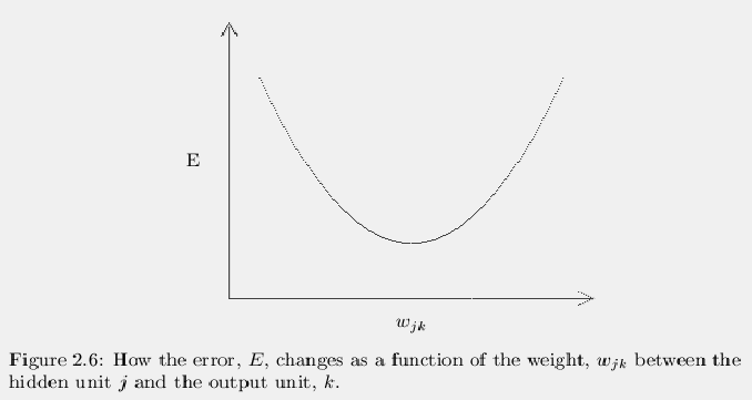
This final term is the slope of the error curve for one weight, w_jk. A plot of the error will then look something like the curve shown in figure 2.6. If the slope is positive we need to decrease the weight by a small amount to lower the error and if the slope is negative we need to increase the weight by a small amount. To move farther down the error curve we can then make the weight change as:

wjk ¬ wjk + (-h) (-(tk - ok) ok(1 - ok) oj)

and the minus signs cancel out¹. People usually define the error signal, d_k as follows:

dk = (tk - ok)ok(1 - ok)

and then the formula for weight changes for weights leading into the output layer becomes:

Dwjk = hdk oj.

Now we have to look at the second part of the problem that relates the change in E to the change in the weight, w_ij. In this case, a change to the weight, w_ij, changes o_j and this changes the inputs into each unit, k, in the output layer. The change in E with a change in w_ij is therefore the sum of the changes to each of the output units. The chain rule produces:

¶E ¶wij = å k  ¶E ¶ok ¶ok ¶netk ¶netk ¶oj ¶oj ¶netj ¶netj ¶wij

= å k  -(tk - ok)ok(1-ok)wjkoj(1-oj)oi

= å k  -dkwjk oj(1-oj)oi.

= -oioj(1-oj) å k  dk wjk

= -oi dj

if we let d_j be:

= oj(1-oj) å k  dk wjk

With this definition the weight change can be written:

Dwij = hdj oi.

These derivations can be generalized to networks with more than 3 layers. The result is the following set of formulas. The first one specifies the weight changes for weights leading into unit j, no matter what layer unit j is in:

Dwij = hdjoi.

The second formula specifies the error signal for the output layer:

dj = (tj - oj) oj (1 - oj).

The third formula specifies the error signal for unit j, in a hidden layer with units k, above:

dj = oj(1 - oj) å k  wjk dk.

Footnotes:

¹Notice the one minus sign before h was introduced to make the error go down and it cancels with the minus sign in the slope term. Then in doing the code the minus sign in the slope term can be ignored if the minus sign with the h is also ignored and that is what has been done in this code. For some weight update methods the minus sign is added later.